Bigtable at Twenty: What Stayed and What Got Rebuilt

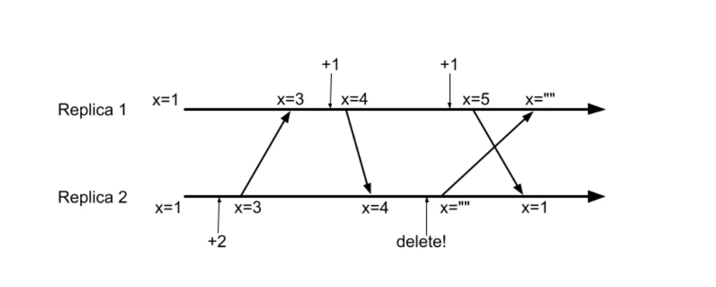
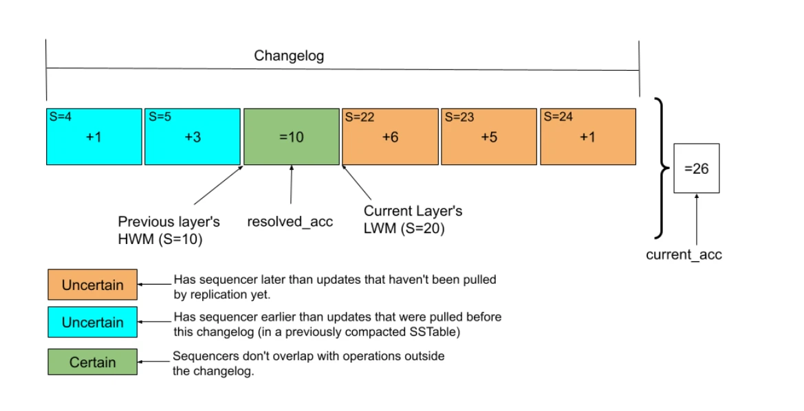
SIGMOD Companion ’26 has a 13-page paper by more than 50 Google authors revisiting Bigtable two decades on. 10 EB, 7 billion QPS, and an architecture that barely moved. This is my reading of why.

SIGMOD Companion ’26 includes a paper called Twenty Years of Bigtable. It has more than 50 Google authors and runs 13 pages. The paper revisits the 2006 OSDI Bigtable paper two decades later: what got added, what got taken apart, and what went wrong in production.

Papers like this are much rarer than new-system papers. In the related work section, the authors point out that more than 200 non-relational data stores have appeared over the past twenty years, but almost nobody writes about running one system for a long time and evolving it along the way. The only comparable accounts they could find are the DynamoDB paper and the Presto paper, and both cover about ten years.

Here is the scale today:

Bigtable manages 10 EB of data at a peak total of 7 billion QPS. A single table can hold more than 1.6 quadrillion rows and more than 1 EB of data; a single cluster peaks above 250 million QPS. Virtually every product area at Google uses it, across thousands of internal teams.

Despite that growth, the core architecture has changed very little. That is the part I wanted to understand.

Off the write path

One sentence in the paper roughly holds the whole twenty years together:

Many of the newer features depend on asynchronous processing that is not on the foreground write path.

Replication works this way. So do CRDT counters. So do materialized views.

This is not an argument that asynchronous processing is inherently better. It moves coordination, computation, and failure recovery out of write latency. The complexity does not disappear; it relocates. What Bigtable got right is that for twenty years there has always been somewhere to put that work, so new capabilities did not require a redesign of the write path.

First, make state movable

Bigtable does not keep data on the tablet server’s local disk. It keeps it in Colossus, the cluster-level file system that succeeded GFS. Moving a tablet therefore does not move data; it just hands the tablet to another server.

The cost is obvious: every read goes through a network file system. So is the benefit: compute and state are separate, and a tablet becomes a scheduling unit you can detach and hand to another machine.

Autoscaling, load balancing, external compaction, and offline access all depend on that decision. If the data were pinned to local disks, every one of those would have been much harder. We made the same bet in GreptimeDB, where compute and storage are decoupled and a region migration hands the region to another datanode without copying any data.

Metadata got the same treatment. Bigtable stores its metadata in its own tables and keeps only the bootstrap information needed to locate the first metadata tablet in Chubby, Google’s lock service. The system manages itself, with very little external state to maintain separately.

Both decisions were already in the 2006 paper. In retrospect, what matters about them is not the work they saved at the time but the doors they left open twenty years later.

Why replication exists

Replication is the single biggest capability added since the original paper. Most users turn it on today. Replicating across dozens of replicas is not uncommon, and the largest user runs more than 200.

The paper frames replication as what makes Bigtable globally available, which many services require. In practice, Google’s internal usage falls into three patterns.

The first is isolating high-throughput traffic from low-latency traffic. The same data often has to serve user-facing reads and writes, shopping data for example, while also feeding batch analytics pipelines. The answer is to point low-latency requests at the primary replica and high-throughput jobs at another, with different cache sizes on each, or even clusters tuned for different service profiles. Teams that do not use replication have to approximate the same effect with offline access or request priorities.

The second is multiple primaries. Plenty of applications do not need cross-row ACID. Put one user’s data in one row, pin that user’s session to one replica, and per-replica per-row ACID is enough. Users typically come from a fixed geography, so local reads and writes are fast, and the data still replicates elsewhere for redundancy.

The third is failover. Long-running pipelines use a replica as intermediate storage, with a secondary standing by. When the primary has a problem, replay whatever was written past the standby’s replication watermark and the pipeline picks up again.

What users need is not merely extra copies. They need to serve the same data under different latency, throughput, and availability requirements. Eventual consistency lowers cost and latency, raises throughput, and allows a write to succeed on one replica. Teams that can design around eventual consistency often find that a good trade.

That first pattern is where we landed too, by a different road. GreptimeDB isolates workloads with replicas as well: read replicas absorb analytical scans while the leader keeps serving low-latency traffic, which is the same division of labor Bigtable users get out of replication. What differs is the bargain underneath. A read replica here holds no copy of its own; it replays the WAL and syncs the manifest over shared object storage, so it stays strongly consistent rather than eventually consistent. For observability workloads I think that is the better trade, but the shape of the answer is the same.

Replication does not coordinate writes

The design is direct: replicas do not coordinate the admission of a mutation. A write that succeeds on one replica is a successful write. The system gets high availability and pays for it with eventual consistency.

Replication uses a pull model. Destination replicas fetch from source replicas rather than sources pushing to every destination. That keeps load off the source, and it leaves each destination tracking its own progress. When a pulling tablet server crashes, it restarts and resumes from where it left off. Under a push model, the source would have to track how far every destination had gotten, and recovery would be more complicated.

Replication runs at the lowest priority, best effort, off spare resources. It is deprioritized relative to user requests and throttled on CPU and memory so background replication cannot push a machine into OOM.

In practice, most data replicates within a minute, but that minute is not a promise. Users who need lower latency can raise the priority or relax the throttles. The system exposes a knob instead of deciding one SLA for everyone. I think that is the right call.

There is also a small, practical detail: roughly once a minute, the system writes a dummy mutation on every replica. Even for a table with no user writes at all, the replication watermark keeps advancing. Otherwise, a cold table’s watermark would sit still, and from outside you could not tell whether it had caught up or the replication path had stalled.

Asynchrony has a concrete downside too.

Say replicas A, B, and C each hold v1, and the GC policy keeps one version. A user writes v2 to A. B reclaims v1 before it has seen v2. C may then receive the deletion of v1 from B before it receives v2 from A. Between those two pulls, C holds no version at all.

So GC cannot look only at local state. When reclaiming by version count, only versions already replicated to every other replica count toward the limit. Age-based GC is not subject to this constraint.

Replication is sound on its own. GC is sound on its own. Together they can briefly lose data. Moving coordination off the write path does not delete the problem: every background mechanism you add has to be checked against the ones already there, and those interactions are the easiest ones to miss.

Bigtable starts doing computation

Bigtable used to be closer to pure storage, with computation handed off to MapReduce, Flume, Beam, or Spark. In recent years, it has taken on SQL, CDC, CRDT counters, and materialized views itself.

These four share an origin: Google Cloud customers asked for them first. Cloud and internal customers run on exactly the same backend, so requirements from the cloud side became part of the core system.

Start with SQL. The motivation was a change in usage. Many teams use Bigtable as a high-throughput ingestion layer, transforming raw data into structured formats for downstream analytics. The data in the middle is often nested JSON, Protobuf, or Avro. Querying it requires granular attribute access rather than pulling a whole row and parsing it yourself. SQL is expressive and widely understood, so it became the primary interface.

The dialect is GoogleSQL. My favorite piece here is row key schemas.

Engineers used to pack several fields into a row key, separate them with delimiters, and express hierarchy by hand inside a one-dimensional key space. The encoding lived entirely in team convention; Bigtable saw a string of bytes.

Row key schemas make that encoding explicit in the system. The components of a row key get types, the SQL engine parses them directly, and range scans and predicate pushdown can target an individual segment. A workaround that users kept reinventing became a first-class capability. That is a pragmatic move.

CDC has a simpler motivation: give users every mutation on their table in real time for applications such as real-time analytics, data synchronization, and fraud detection.

The CRDT section is more involved.

It exists because users had no good option. To maintain a counter in Bigtable, you previously had two choices. One was a generic read-modify-write transaction: expensive, hard to scale, and incompatible with asynchronous replication, since replication ships individual cell value updates rather than coordinated cross-cell operations. The other was to store every delta separately and either aggregate at read time or run another external background job to fold deltas into a summary. The paper says outright that part of why Redis and Cassandra are popular here is that they offer a lightweight answer.

The technical difficulty is deletion. If you only have commutative operations like increment and decrement, each replica can keep its own running total. Clearing a counter is not commutative, so the same set of operations arriving at different replicas in different orders produces different results.

Figure 2 from Fabio Baltieri et al., “Twenty Years of Bigtable”, SIGMOD Companion ’26. Both replicas start at 1 and both receive +2, +1, +1, and one delete, only in different orders. Replica 1 has already reached 5 when the delete arrives and gets cleared; Replica 2 is cleared first and only then receives that +1, so it lands on 1.

The paper notes in passing that Redis and Cassandra both have constraints or extra procedures around deleting counters, while Bigtable wanted deleting CRDT data to be no different from deleting anything else.

The solution is embedded directly in the LSM tree. Each layer holds a resolved subtotal plus a log of operations that are not yet resolved.

Figure 3 from Fabio Baltieri et al., “Twenty Years of Bigtable”, SIGMOD Companion ’26. The green resolved_acc=10 in the middle is the part already folded in, which can no longer overlap with anything elsewhere; the three orange entries on the right are recent updates replication has not caught up with; the two cyan entries on the left are late arrivals. All six sum to current_acc=26.

Trimming, which folds the log into the subtotal, happens during merge compaction. Deletes close out here as well: when a tablet server processes a delete, it directly removes operations sequenced before it from the memtable’s changelog, and every later trimming pass drops operations sequenced before the most recent delete observed.

Materialized views solve an operational problem. Bigtable usually has pipelines hanging off it that derive secondary data from a primary source, from simple secondary indices to complex analytical rollups. That used to mean MapReduce or Flume, and after CDC arrived, streaming engines like Dataflow. But an external pipeline has a separate resource quota and upgrade path, plus end-to-end consistency to maintain across two systems. Moving the derivation logic into the database removes those operational boundaries; the user writes one SQL statement.

The implementation reuses existing mechanisms. When the source table is updated, the tablet server records the local logical clock in a hidden column, and a server-side mapper -> shuffle table -> reducer -> finalizer pipeline runs from there. Each stage tracks its progress with a watermark.

This is the section I read most carefully, because GreptimeDB’s Flow engine has the same shape: a foreground write only marks a dirty window, the aggregation runs asynchronously on flownodes, and progress is tracked with region watermarks and checkpoints. Our incremental query RFC is where that design is being argued out.

CRDTs borrowed LSM compaction. Materialized views borrowed the logical clocks and watermarks replication was already using. Both features build on existing mechanisms, and neither required a change to the foreground write protocol.

When I judge how long a storage architecture will last, the first practical question I ask is: when the next major feature arrives, where does it attach?

If the answer keeps being “you rewrite the main read or write path,” the system will eventually be crushed by its own history.

Correctness runs in the background too

The same approach shows up in data integrity. The premise is straightforward: at Bigtable’s scale, any conceivable hardware or software error will happen. The goal is to make undetected corruption sufficiently unlikely.

Bigtable checksums at several granularities with CRC32: row keys, column keys, and values, plus a file-level checksum on every file. Users can supply their own CRC32C on write, and if they do not, the client library generates one. These get validated when the RPC arrives, before the commit log write, before the memtable update, and along the replication path.

The expensive part happens later. After an SSTable is built but before it is recorded in metadata, the whole thing is read back: decrypted, uncompressed, parsed entry by entry, with every checksum verified again. File builder jobs do that work outside the tablet servers. The paper says it is resource intensive and reports that virtually no SSTable inconsistencies have been observed in years.

Section 7 states the tradeoff directly: the extensive use of checksums costs resources and is paying off.

The write path only does the checks that can finish immediately. File builders and compaction handle the expensive full read-back. Correctness follows the same pattern as the newer features, and it is the item on this list I most want to steal.

The architecture held, but the internals changed

A stable architecture does not mean nothing changed inside for twenty years. As scale grew, work was parallelized where possible and moved out of the stateful service when it did not need to run there.

Bigtable’s master is a single-process control plane. After tablet counts rose by orders of magnitude, the master hit lock contention, and the data structures that manipulate tablets had to move to fine-grained locking.

Schema updates used to run serially. As schemas grew more complex, clusters grew larger, and changes became more frequent, serial execution stopped being acceptable, so it was parallelized.

File GC changed the most visibly. In 2006, the master ran mark-and-sweep serially. Now the heavy work, including reading metadata tables, writing intermediate state, listing files, and issuing deletes, is done in parallel by tablet servers. The master only divides the work and collects results. A full pass takes minutes to tens of minutes.

Other work moved out of the service.

External compaction hands SSTable building to independent jobs that scale on their own. Location cache proxies absorb location lookups on behalf of the metadata servers. Offline access lets batch workers read SSTables on Colossus directly, mostly bypassing Bigtable’s servers, and lets them use cheaper, throughput-oriented CPUs; Cloud Bigtable’s Data Boost is built on this. Bulk import goes furthest: workers build SSTables directly, and afterward tablet servers update the metadata and claim the files.

The principle is familiar: work that scales independently and does not need to hold core state should move out of the stateful service. Applying it one piece at a time inside a twenty-year-old system, without pulling the system apart, is the difficult part.

The stable architecture comes with a bill, though.

Bigtable still offers only single-row transactions. Data that must be updated atomically has to be packed into one row, so some tables grew very large rows, which bring performance problems of their own. The paper advises applications to revise their logic and avoid writing data that way.

That tradeoff dates to 2004 and still makes users change application code today. All the earlier upside came from the architecture not changing, and so does this one. The complexity did not disappear; it relocated, and this time it landed on the user.

Resource efficiency became a product capability

I had not expected this section. The paper devotes a whole section to resource efficiency. While discussing SQL versus non-relational models, it notes that scalability and performance are usually treated as the selling points of non-relational databases, but in Google’s experience, resource efficiency is just as much a reason users pick Bigtable.

Autoscaling comes in two layers.

Inside the cluster, an autosizer runs on a sub-minute frequency, adding and removing machines from a pool of idle servers called the slack subpartition. Only when that pool runs dry or sits idle too long does the system call company-wide autoscaling for machines from a central pool.

Speed is the first reason. Servers in the slack pool are under the master’s own control and can be brought in quickly, while central provisioning can take several minutes.

The second reason is that a database knows what actually counts as running short. CPU and memory are surface metrics; domain signals like tablet availability feed into the decision too, and a generic autoscaler cannot see them.

The cache has its own sizer. It uses a total-cost-of-ownership model to set each server’s cache limit dynamically, because cache benefit has a distinct knee. Past that point, more memory buys almost no performance and just costs money.

At 10 EB, saving resources is not a line item in a finance report. It is part of what the database is good at.

Two counterintuitive details

When you deal with a hotspot, moving the hottest tablet is usually the wrong move.

Every client has its old location cached. The moment the hot tablet moves, a wave of requests discovers a stale cache and turns into location lookups. Bigtable leaves the hottest tablet where it is and moves colder neighbors instead. In extreme cases, a tablet server ends up hosting nothing but that one hotspot.

The other one is Bloom filters.

Bigtable’s Bloom filters were badly underused for a while. The cause was not a deep algorithmic issue. The implementation required the filter condition to include both a column family and a column, and a large share of users query by column family only, so the filter did not apply.

A hybrid mode raised utilization by 4x at under one percent additional disk footprint.

Some workloads look up keys that are almost always present, where consulting a Bloom filter is wasted work. Bigtable periodically evaluates whether a filter is still useful and turns it off when it is not.

I like both of these. In a mature database, a lot of the wins come not from refining the algorithm but from admitting that real workloads do not behave the way the designers imagined.

Who runs Bigtable

Bigtable was originally meant to be run by each user team. Not long after launch, Google found that most teams did not have the expertise to maintain it. From mid-2006 onward, Bigtable became a company-wide service owned by a dedicated SRE team. Today, almost all usage sits inside that service, and only a small number of teams still run their own clusters.

There is a design in the monitoring section I like. Alongside the metadata prober, which reads metadata rows one by one looking for unavailable ranges, each cluster runs a blackbox latency prober that the paper describes as aiming to mimic a well-behaved Bigtable user. It runs a fixed workload against a dedicated table in every partition, exports read and write latencies, and feeds those measurements into the latency SLIs and alerting.

You do not know how real users will abuse the system, so start by making a well-behaved user’s experience measurable.

The paper closes by noting that a Bigtable this large can be managed by a relatively small team of SREs with sufficient domain knowledge.

Put that beside the reason the service exists in the first place, that most teams could not run Bigtable themselves, and the conclusion is hard to avoid. Operability is part of the architecture, not something outside it. A system that only its authors can run will not last twenty years, however elegant the design.

I expect to reread this paper a few more times. It leaves me with two questions for GreptimeDB.

First, do the background jobs we run, including compaction, flush, and index building, carry the same interaction risk as replication and GC? Each mechanism may be sound on its own while violating an implicit assumption when combined with another.

Second, how often have our major features forced a change to the main read or write path?

I do not know the answer to the second one yet.

References

1. Fabio Baltieri et al., “Twenty Years of Bigtable”, SIGMOD Companion ’26. DOI: 10.1145/3788853.3803095